Playing with a NavSpark and R
Back in January I managed to get in early on the Indiegogo campaign for the NavSpark GNSS receiver. For no real reason other than the fact that it was US$17 including shipping, I decided to buy one of the NavSpark-BD boards. Besides being an Arduino-compatible board with built-in GPS, this version is also able to pick up satellites from the Chinese Beidou constellation.
While the modified Arduino client isn't available for OS X (according to the FAQ, the LEON3 chip in the NavSpark doesn't have an OS X cross-compiler available), I decided to have a look at some of the GPS data just to see what I could pick up. This StackExchange answer has been really useful for connecting to serial devices over USB, and the NavSpark uses the PL2303 chip which has an open-source driver available for OS X.
After installing the driver, I found the NavSpark port using ls /dev/tty.*. Since the default baud rate is 115200, screen /dev/tty.NoZAP-PL2303-000012FD 115200 started showing the GPS data from the Navspark in NMEA format. There are plenty of places that this format's described, but the NavSpark resources page has an easy-to-read PDF. Using the lines starting with $--GSV and $--GSA, I decided to see if I could plot where the satellites were using R.
After the board had been running for a while I got the following lines:
$GNGSA,A,3,05,07,10,28,26,08,,,,,,,2.7,1.6,2.1*28
$GNGSA,A,3,207,,,,,,,,,,,,2.7,1.6,2.1*18
$GPGSV,4,1,13,30,72,208,33,10,70,316,19,08,70,194,35,07,51,149,30*71
$GPGSV,4,2,13,28,42,006,21,05,36,230,21,13,33,095,12,26,15,240,26*79
$GPGSV,4,3,13,02,14,289,,04,09,326,,03,07,120,,23,06,075,*70
$GPGSV,4,4,13,19,02,105,*45
$BDGSV,2,1,08,209,73,292,,207,71,222,30,210,57,265,,206,55,004,*67
$BDGSV,2,2,08,203,52,348,,201,46,040,,208,02,016,,213,00,272,27*61
The third number in each GSV line indicates that there were 13 GPS (GP) and 8 Beidou (BD) satellites visible - not bad considering there were three layers of concrete between the antenna and the sky when I was testing this! As I was just working with the above data, I entered the satellite elevation and azimuth data by hand this time around:
azimuth <- c(208, 316, 194, 149, 6, 230, 95, 240, 289, 326, 120, 75)
azimuth.bd <- c(292, 222, 265, 4, 348, 40, 16, 272)
elevation <- c(72, 70, 70, 51, 42, 36, 33, 15, 14, 9, 7, 6)
elevation.bd <- c(73, 71, 57, 55, 52, 46, 2, 0)
After I'd grabbed this data, I used polar.plot() from the plotrix package to visualise the position of the satellites (this satellite location data is from 2014-05-24 at 13:33:59 UTC). I made up two additional vectors (used and used.bd) that contained the numeric values corresponding to open and closed circles. Since these were entered in the order that I'd entered the azimuth and elevation data, they could be passed to the point.symbols argument to show which satellites were being used to give a fix.
polar.plot(90 - elevation, azimuth, rp.type = "s", radial.lim = c(0, 90, seq(0, 90, 15)), start = 90, clockwise = TRUE, show.grid.labels = FALSE, labels = compass, label.pos = seq(0, 337.5, 22.5), point.symbols = used)

radial.plot(90 - elevation.bd, azimuth.bd, rp.type = "s", radial.lim = c(0, 90, seq(0, 90, 15)), start = 90, clockwise = TRUE, add = TRUE, point.symbols = used.bd, point.col = "red")
The end result was this (Beidou satellites in red, GPS in black):
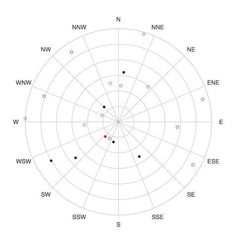
I'm quite pleased with this for something that came out of my first evening of hacking in quite a long time. With a better set of functions to process the NMEA data coming from the NavSpark, it should be possible to see how the satellites move over time, much as has been done in this post by Gergely Imreh. I'm hoping to try something like this in the future - perhaps it can be a project for the next long weekend.